Build a LLM (1/2)
It's a journey into the heart of modern AI, where you'll learn about data preprocessing, model architecture, and the fascinating process of training a model to understand and generate human-like text.

This post is based mainly on my own experience while following the steps in the book, "Build a Large Language Model (from scratch)" by Sebastian Raschka.
Large Language Model in short
There are already too many definitions for this term. So in short, we could think it like a machine software that is able to response to human-like text. LLMs utilizes Transformer architecture which allows them to predict the output based on the attention to different parts of the input.
Stages of building and using LLMs
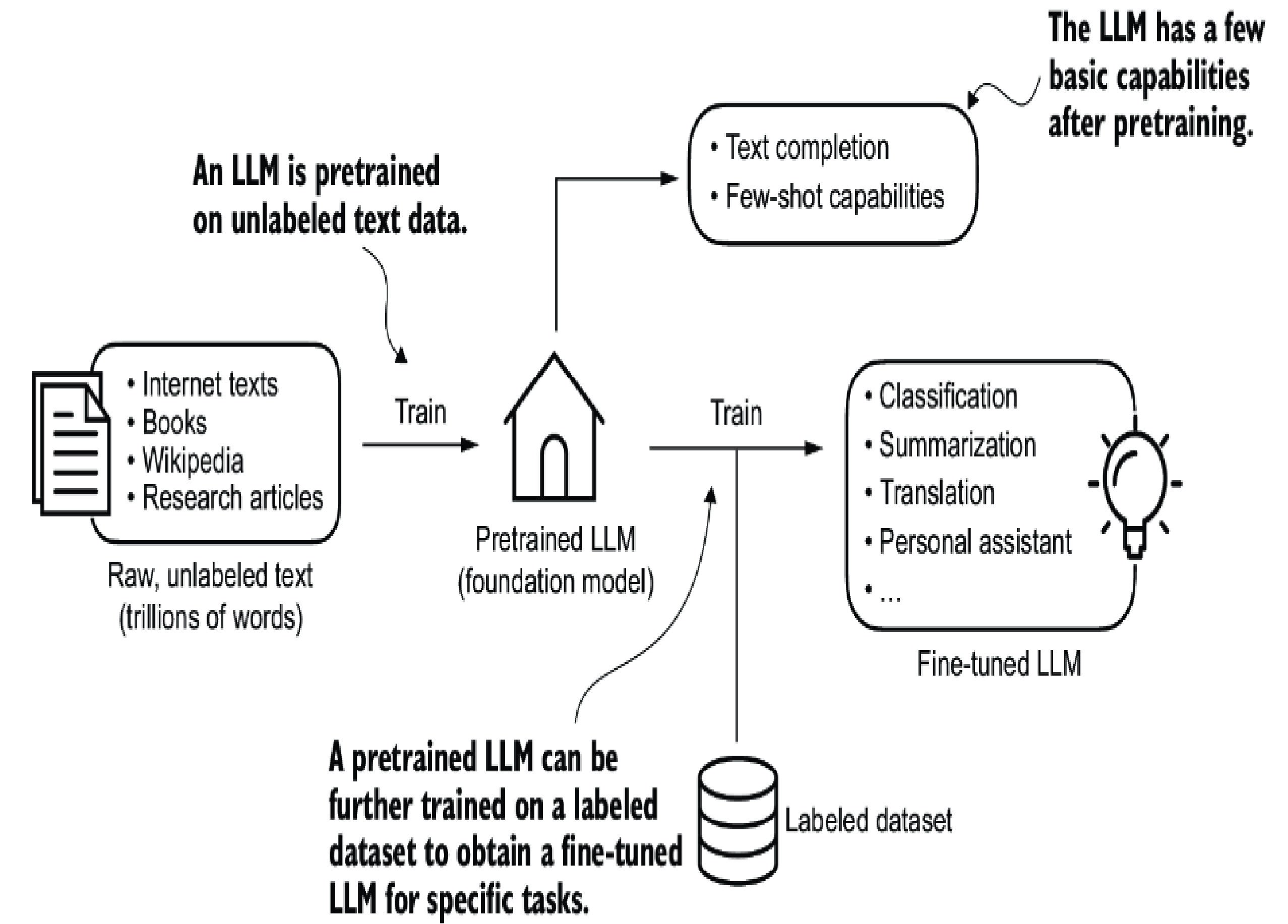
There are 2 most popular categories of fine-tuning LLMs are:
- Instruction fine-tuning: the labeled dataset consists of instruction and answer pairs.
- Classification fine-tuning: the labeled dataset consists of texts and associated class labels. (for ex: "spam" and "not spam" labels)
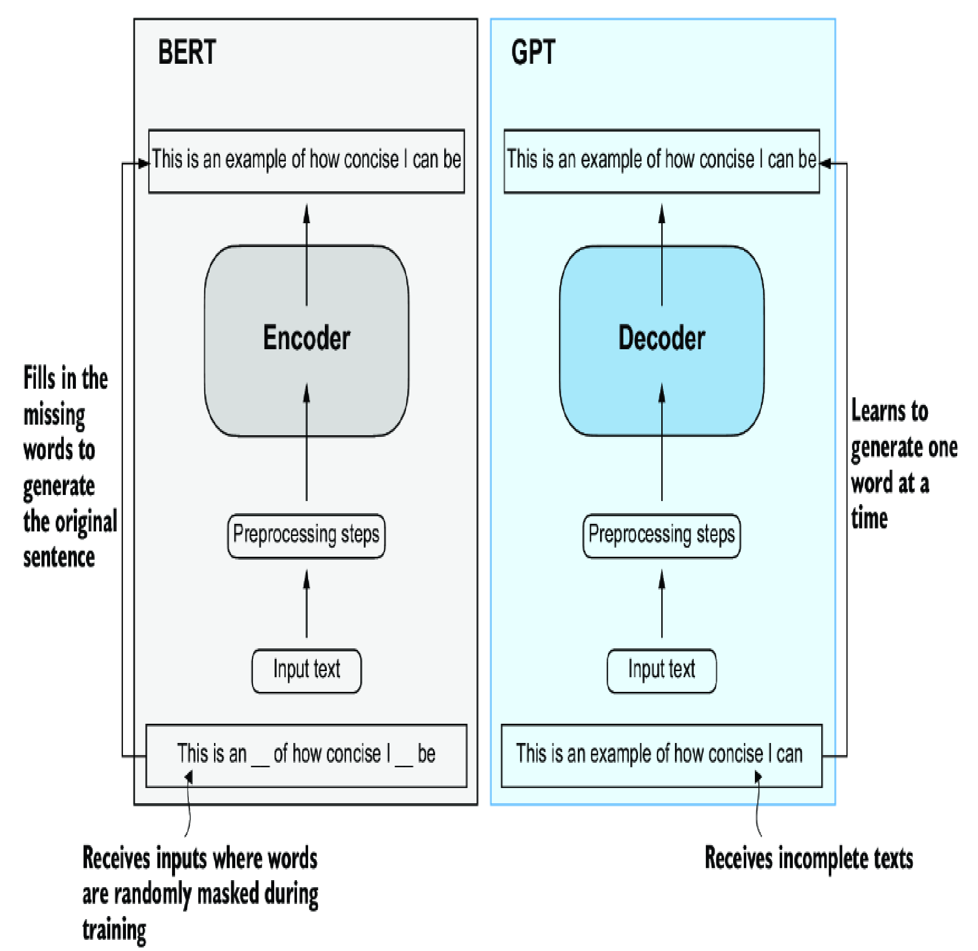
Transformer architecture
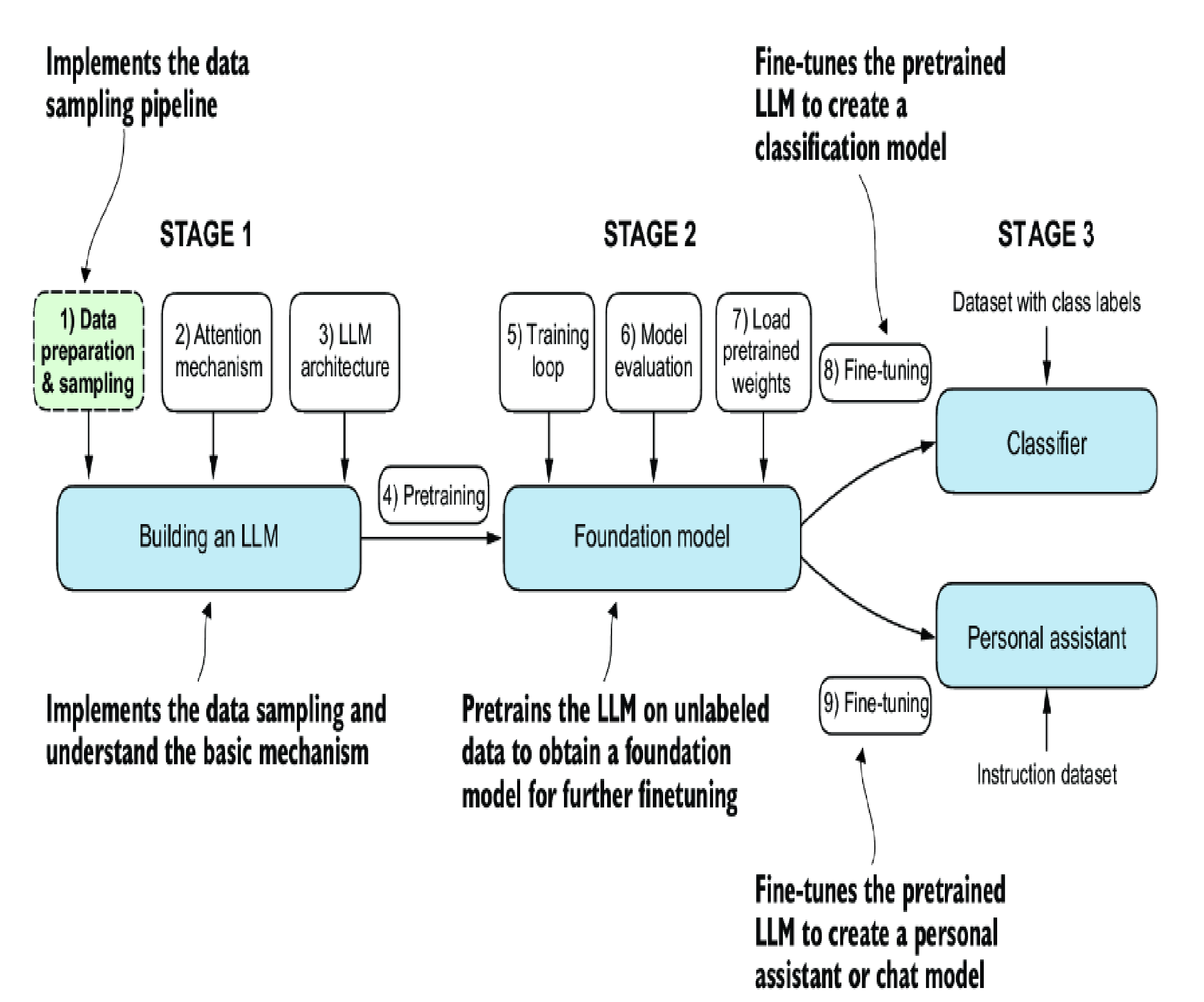
Training LLMs process
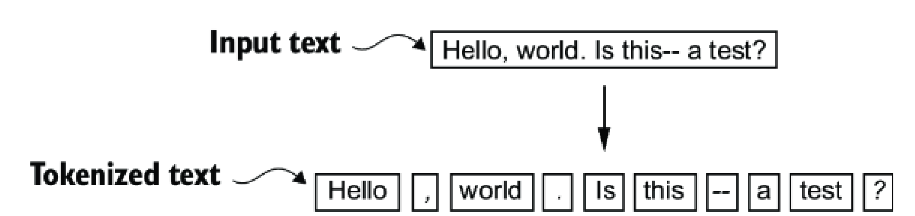
Data preparation
Machine is not human, hence it needs to convert human texts into vectors for it to process. To to that, first we split the text into tokens:
Then we convert those tokens into vectors, something likes: [ 0.3374, -0.1778, -0.1690] (this is 3-dimension vector, in reality it could be thousands of dimensions, for ex: GPT-3 used 12,288 dimensions)
However, if we only converting text into tokens, then the LLM will only understand the word itself but could not differentiate the position of the token which creates a context with others sibling words (of course only us, human, could understand the context). So we will enrich those vectors with position vectors: absolute or relative positional embeddings.
When saying embeddings, we mean it to be "add" operation.
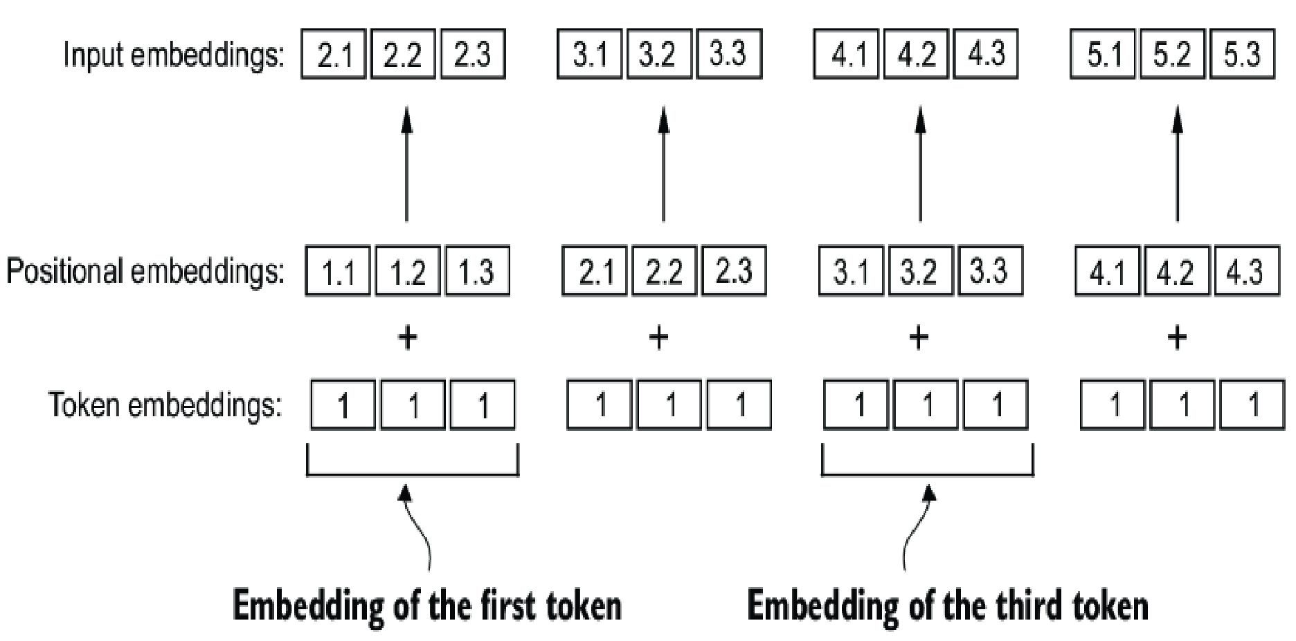
Above is the illustration of the same token (vector: [1,1,1]) now can be embedded with position vectors to be different vectors (top row), which is supposed to have "context".
Runnable code
import tiktoken
import torch
from torch.utils.data import Dataset, DataLoader
import os
import urllib.request

class GPTDatasetV1(Dataset):
    def __init__(self, txt, tokenizer, max_length, stride):
        self.input_ids = []
        self.target_ids = []

        # Tokenize the entire text
        token_ids = tokenizer.encode(txt, allowed_special={"<|endoftext|>"})

        # Use a sliding window to chunk the book into overlapping sequences of max_length
        for i in range(0, len(token_ids) - max_length, stride):
            input_chunk = token_ids[i:i + max_length]
            target_chunk = token_ids[i + 1: i + max_length + 1]
            self.input_ids.append(torch.tensor(input_chunk))
            self.target_ids.append(torch.tensor(target_chunk))

    def __len__(self):
        return len(self.input_ids)

    def __getitem__(self, idx):
        return self.input_ids[idx], self.target_ids[idx]

# this method use tiktoken or BytePair encoding tokenizer
def create_dataloader_v1(txt, batch_size, max_length, stride,
                         shuffle=True, drop_last=True, num_workers=0):
    # Initialize the tokenizer
    tokenizer = tiktoken.get_encoding("gpt2")

    # Create dataset
    dataset = GPTDatasetV1(txt, tokenizer, max_length, stride)

    # Create dataloader
    dataloader = DataLoader(
        dataset, batch_size=batch_size, shuffle=shuffle, drop_last=drop_last, num_workers=num_workers)

    return dataloader

if __name__ == "__main__":

    if not os.path.exists("the-verdict.txt"):
        url = ("https://raw.githubusercontent.com/rasbt/"
            "LLMs-from-scratch/main/ch02/01_main-chapter-code/"
            "the-verdict.txt")
        file_path = "the-verdict.txt"
        urllib.request.urlretrieve(url, file_path)

    with open("the-verdict.txt", "r", encoding="utf-8") as f:
        raw_text = f.read()

    vocab_size = 50257
    output_dim = 256
    context_length = 1024


    token_embedding_layer = torch.nn.Embedding(vocab_size, output_dim)
    pos_embedding_layer = torch.nn.Embedding(context_length, output_dim)

    batch_size = 8
    max_length = 4
    dataloader = create_dataloader_v1(
        raw_text,
        batch_size=batch_size,
        max_length=max_length,
        stride=max_length
    )

    data_iter = iter(dataloader)
    inputs, targets = next(data_iter)
    print("Inputs:\n", inputs)
    print("\nTargets:\n", targets)

    token_embeddings = token_embedding_layer(inputs)
    print(token_embeddings.shape)

    pos_embeddings = pos_embedding_layer(torch.arange(max_length))
    print(pos_embeddings.shape)

    input_embeddings = token_embeddings + pos_embeddings
    print(input_embeddings.shape)
dataset.py
Attention mechanisms
Self-attention is a mechanism that allows each position in the input sequence to consider the relevancy of, or "attend to," all other positions in the same sequence. In sort, LLM needs to know the importance of the token in the sequence to "understand" the context.
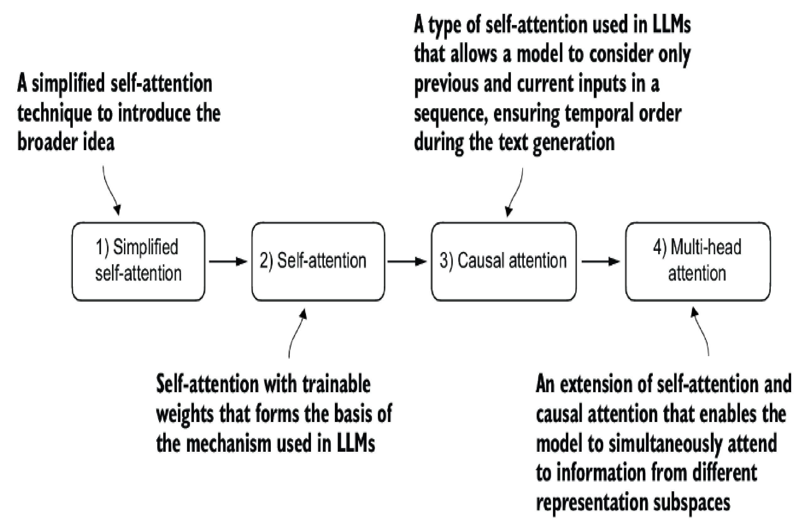
Simplified self-attention
This is not a part of the structure of Transformer block, it is rather the basic idea of the self-attention representation in LLM.
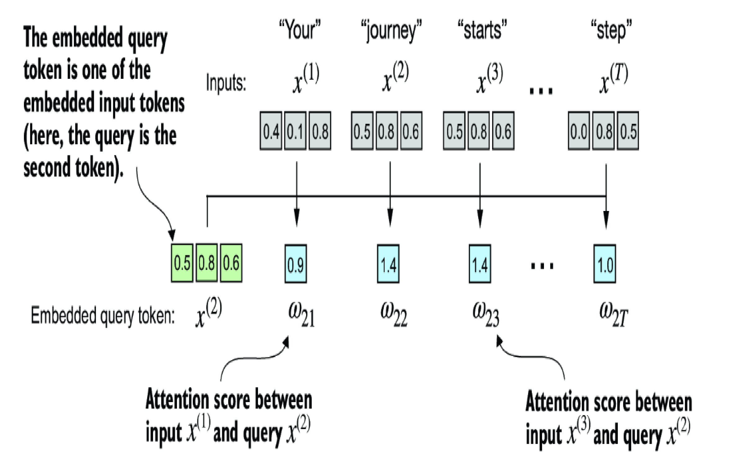
The idea is using dot-product (a method of multiplying two vectors to yield a scalar value) to measure the similarity of the two token. Above example is measuring the vector token 2 (of "journey") "attends to" other tokens in the sequence. The higher value means the two are higher similarity.
The softmax function then is used to normalize those weight \( w_{2i} \) that we calculated above:
\[ \alpha_{2i}=softmax(w_{2i})=\frac{e^{w_{2i}}}{\sum_{j=1}^{n}e^{w_{2j}}} \]
above function will amplify the importance of the token, make sure that total of all weights equals to 1 for easy loss computation.
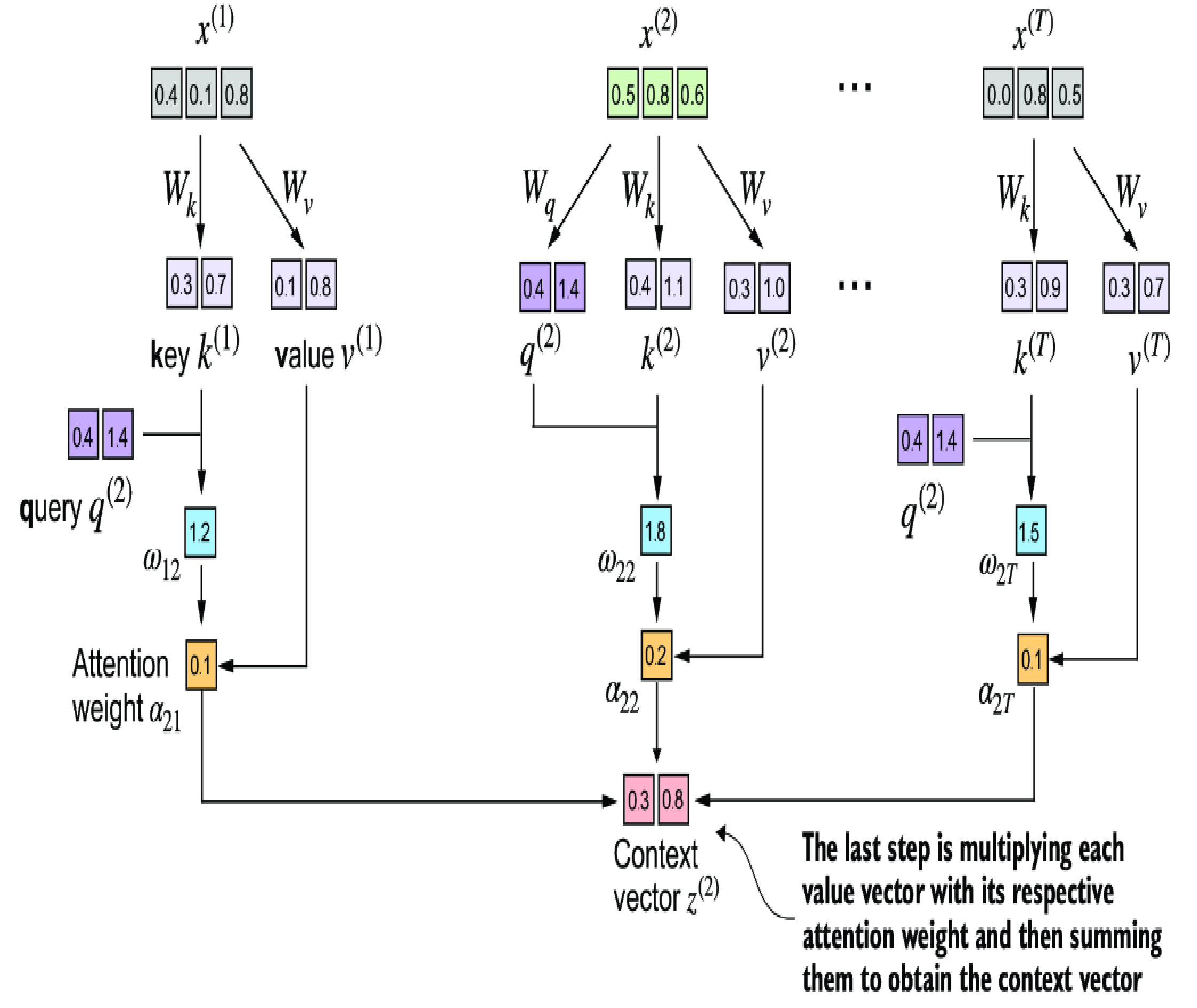
Then these normalized weight \( \alpha_{2i} \) will multiply with token vector and then sum for context vector \( z ^{(2)} \). So now, instead of using \( x ^{(2)} \), we use \( z ^{(2)} \) because it has additional information about the attention of \( x ^{(2)} \) with the rest of the sequence.
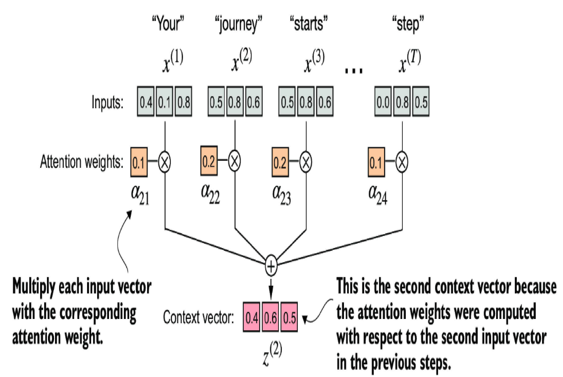
In fact, we don't use \( z ^{(2)} \) as input of any layer, as mentioned earlier, this process is just for understanding the concept. Also, this \( z ^{(2)} \) value is what we want the LLM to learn from the data (target value)
In above example, we calculate the context vector from T input tokens, this T is also the context length of the LLM. For ex, GPT-2 has context length of 1024 means the context vector are calculated based on 1024 input tokens and use that information to predict the next token. If the input data is less than this context length, it will be padded with special token and ignored in self-attention.
Self-attention with trainable weights
In the LLM architecture, instead of calculate the fixed value of \( \alpha_{2i} \) previously, we use trainable weight matrices \( W_{q} \) (like a search query), \( W_{k} \) (like the key used for indexing), \( W_{v} \) (like value of the data). There matrices can be think as the placeholders to hold the learnt parameters of LLM; it will be initialized with controlled random values, and will be adjusted based on the backward propagation of learning process.
Okay, so to be cleared about these matrices, we need to understand the learning process generally: whenever data is feed into the LLM for training, it (after tokenized, vectorized and normalized) will go through the computation process similar to the self-attention concept that we explained earlier in a couple times so that in final output we can determine what is the predicted word. Based on the output we will compare with the expectation and propagate back this difference through layers of the LLM and each layer will make adjustment on those \( W_{q} \), \( W_{k} \), \( W_{v} \), so that it will be better in prediction the next word. This process will be happened trillion times and the final set of values of \( W_{q} \), \( W_{k} \), \( W_{v} \) will be the final model params that we will use for inference.
Runnable code
import torch
import torch.nn as nn

class SelfAttention_v2(nn.Module):

    def __init__(self, d_in, d_out, qkv_bias=False):
        super().__init__()
        self.W_query = nn.Linear(d_in, d_out, bias=qkv_bias)
        self.W_key   = nn.Linear(d_in, d_out, bias=qkv_bias)
        self.W_value = nn.Linear(d_in, d_out, bias=qkv_bias)

    def forward(self, x):
        keys = self.W_key(x)
        queries = self.W_query(x)
        values = self.W_value(x)

        attn_scores = queries @ keys.T
        attn_weights = torch.softmax(attn_scores / keys.shape[-1]**0.5, dim=-1)

        context_vec = attn_weights @ values
        return context_vec


if __name__ == "__main__":

    inputs = torch.tensor(
    [[0.43, 0.15, 0.89], # Your     (x^1)
    [0.55, 0.87, 0.66], # journey  (x^2)
    [0.57, 0.85, 0.64], # starts   (x^3)
    [0.22, 0.58, 0.33], # with     (x^4)
    [0.77, 0.25, 0.10], # one      (x^5)
    [0.05, 0.80, 0.55]] # step     (x^6)
    )

    d_in = inputs.shape[1]
    d_out = 2
    print(f'{d_in}, {d_out}')
    torch.manual_seed(789)
    sa_v2 = SelfAttention_v2(d_in, d_out)
    print(sa_v2(inputs))
self_attention.py
Causal attention
We has understand how the context vector is calculated in LLM, but in reality, we don't want the LLM will be feed with all the data at once, but we want it to predict the next token based on the token we feed into to (incomplete sequence).
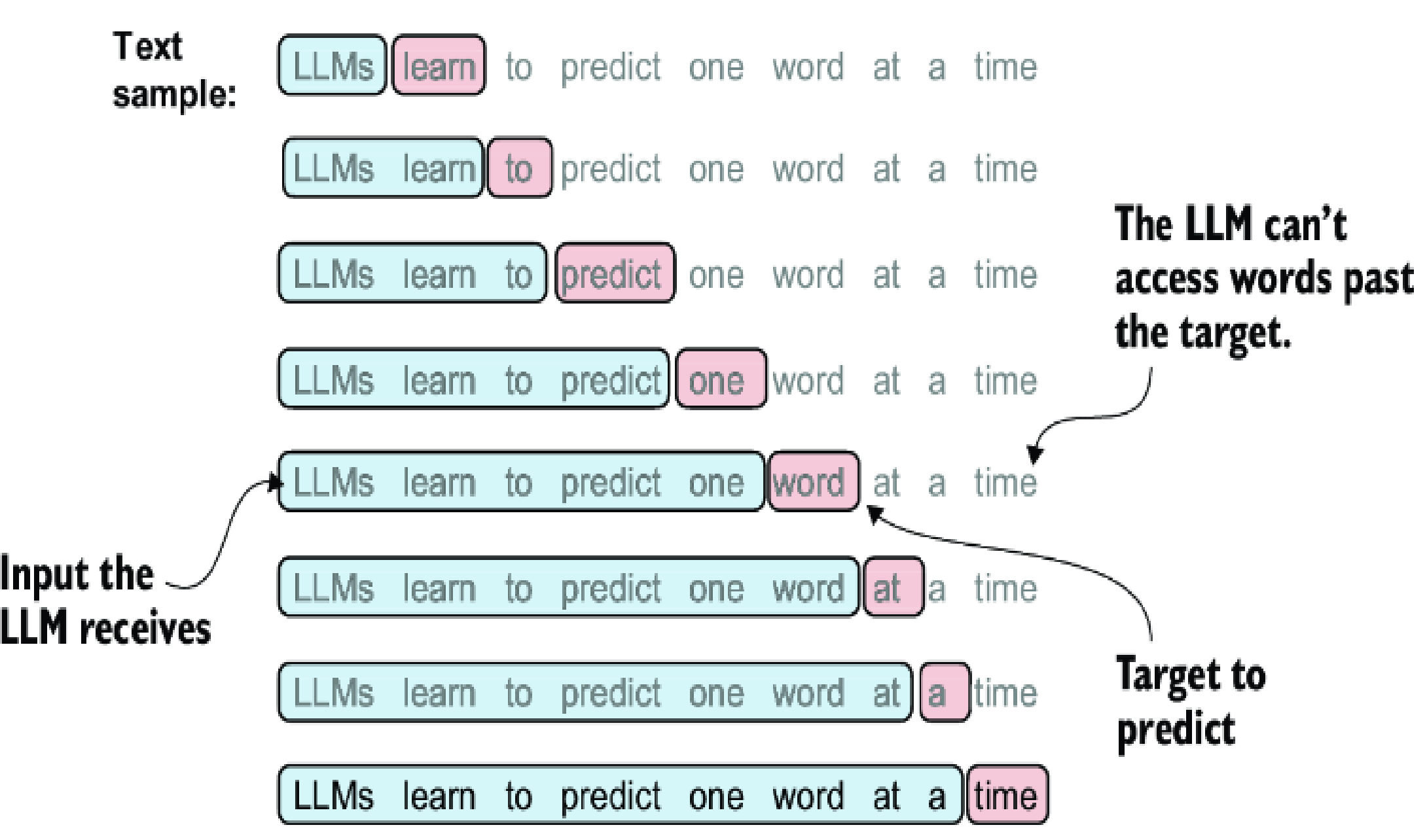
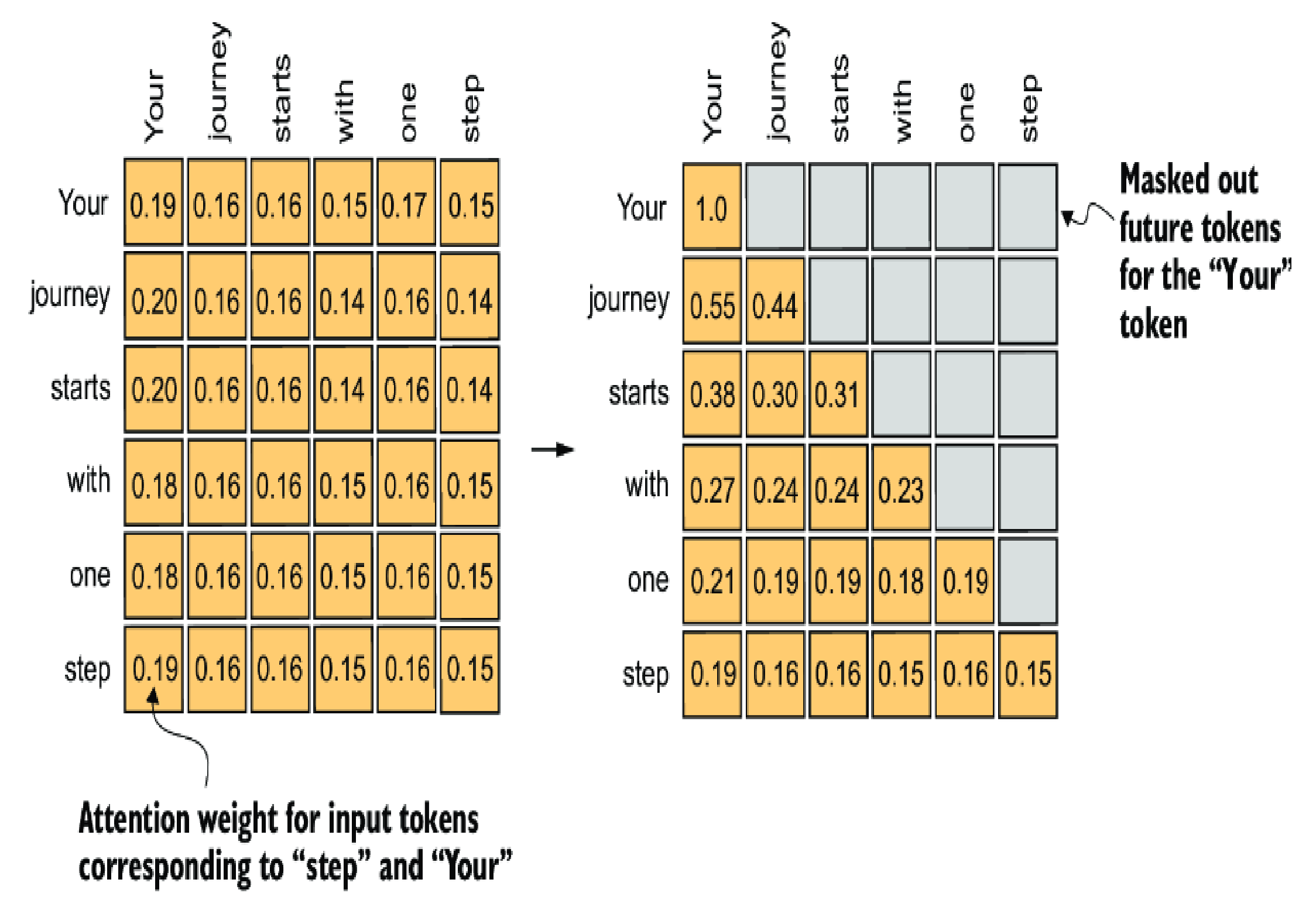
In other to do that, we need to masked out future tokens before feeding to the LLMs
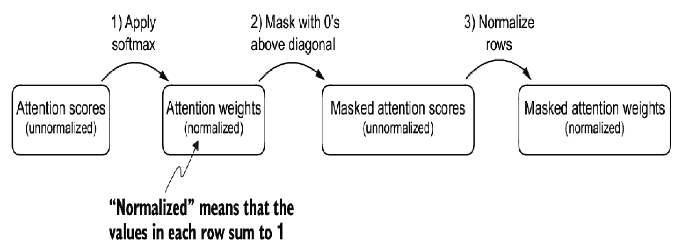
Remember, when masked those attention scores that above the diagonal, we make the matrices become unnormalized (total of a row is not 1 anymore) so a normalization is needed after the masking.
Runnable code
import torch
import torch.nn as nn

class CausalAttention(nn.Module):

    def __init__(self, d_in, d_out, context_length,
                 dropout, qkv_bias=False):
        super().__init__()
        self.d_out = d_out
        self.W_query = nn.Linear(d_in, d_out, bias=qkv_bias)
        self.W_key   = nn.Linear(d_in, d_out, bias=qkv_bias)
        self.W_value = nn.Linear(d_in, d_out, bias=qkv_bias)
        self.dropout = nn.Dropout(dropout) # New
        self.register_buffer('mask', torch.triu(torch.ones(context_length, context_length), diagonal=1)) # New

    def forward(self, x):
        b, num_tokens, d_in = x.shape # New batch dimension b
        # For inputs where `num_tokens` exceeds `context_length`, this will result in errors
        # in the mask creation further below.
        # In practice, this is not a problem since the LLM (chapters 4-7) ensures that inputs
        # do not exceed `context_length` before reaching this forward method.
        keys = self.W_key(x)
        queries = self.W_query(x)
        values = self.W_value(x)

        attn_scores = queries @ keys.transpose(1, 2) # Changed transpose
        attn_scores.masked_fill_(  # New, _ ops are in-place
            self.mask.bool()[:num_tokens, :num_tokens], -torch.inf)  # `:num_tokens` to account for cases where the number of tokens in the batch is smaller than the supported context_size
        attn_weights = torch.softmax(
            attn_scores / keys.shape[-1]**0.5, dim=-1
        )
        attn_weights = self.dropout(attn_weights) # New

        context_vec = attn_weights @ values
        return context_vec

if __name__ == "__main__":

    inputs = torch.tensor(
    [[0.43, 0.15, 0.89], # Your     (x^1)
    [0.55, 0.87, 0.66], # journey  (x^2)
    [0.57, 0.85, 0.64], # starts   (x^3)
    [0.22, 0.58, 0.33], # with     (x^4)
    [0.77, 0.25, 0.10], # one      (x^5)
    [0.05, 0.80, 0.55]] # step     (x^6)
    )

    d_in = inputs.shape[1]
    d_out = 2

    batch = torch.stack((inputs, inputs), dim=0)
    print(batch.shape)

    torch.manual_seed(123)

    context_length = batch.shape[1]
    ca = CausalAttention(d_in, d_out, context_length, 0.0)

    context_vecs = ca(batch)

    print(context_vecs)
    print("context_vecs.shape:", context_vecs.shape)
casual_attention.py
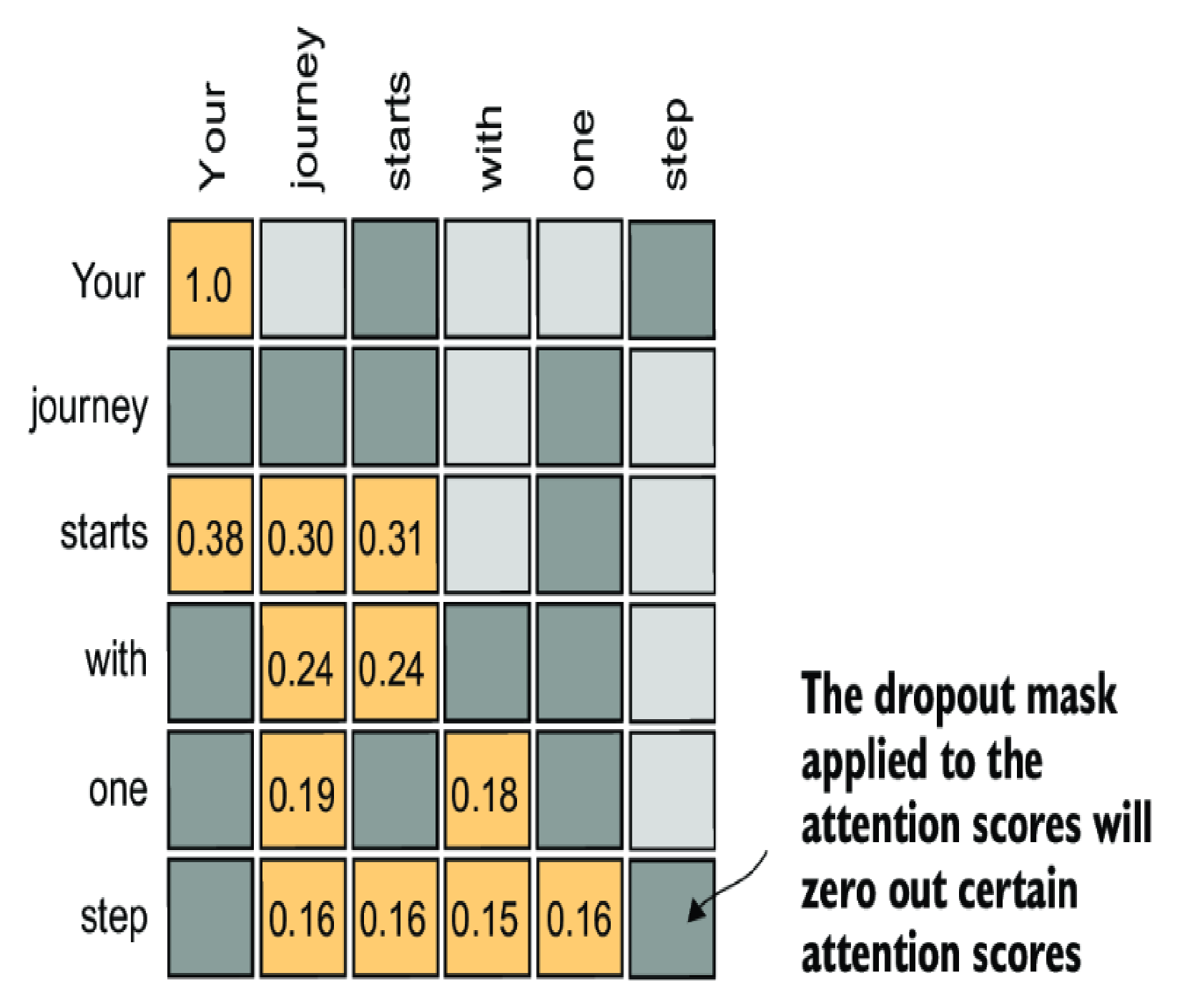
Dropout
Dropout in deep learning is a technique where randomly selected hidden layer units are ignored during training, effectively “dropping” them out. This method helps prevent overfitting by ensuring that a model does not become overly reliant on any specific set of hidden layer units.
It’s important to emphasize that dropout is only used during training and is disabled afterward.
Multi-head attention
In short, we will have many group of \( W_{q} \), \( W_{k} \), \( W_{v} \) to make the LLM learn many aspects of the data.
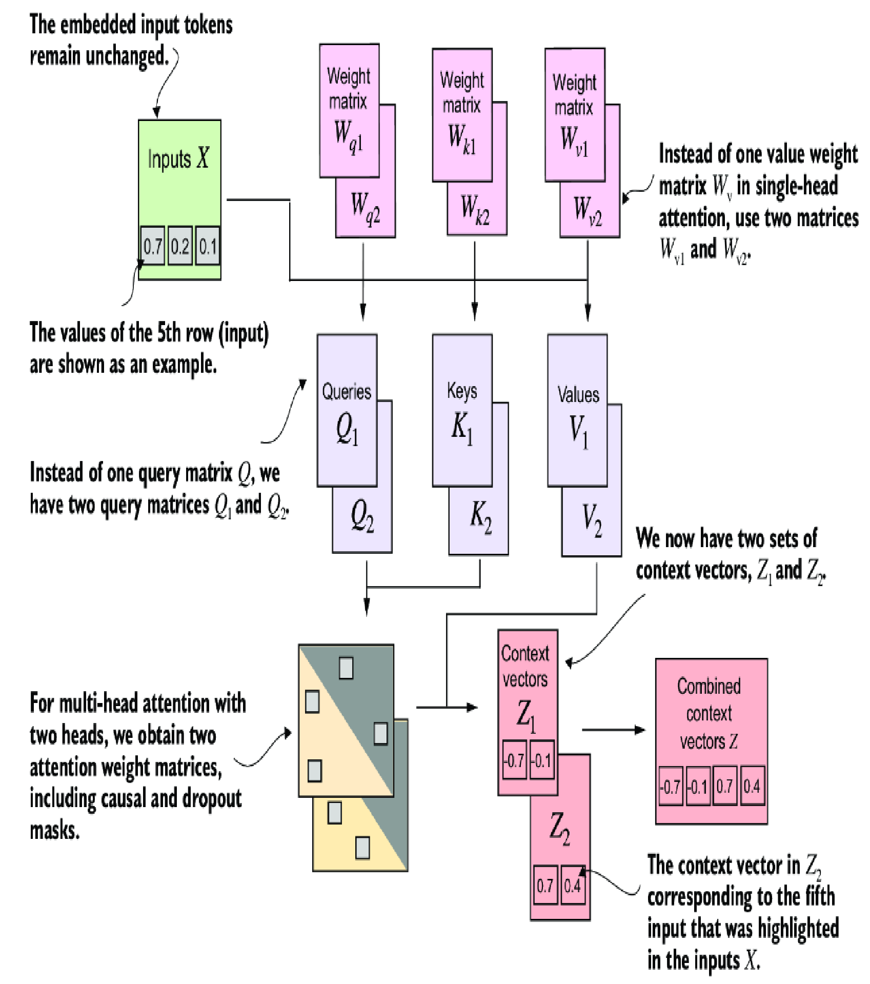
Basically, those \( W_{q2} \), \( W_{k2} \), \( W_{v2} \) are not different from \( W_{q1} \), \( W_{k1} \), \( W_{v1} \) in structure. But they are initialized with different values and get adjusted with different values in the backward propagation process. Because of the independency, each group is consider as a different head to learn different things from the same data.
Runnable code
import torch
import torch.nn as nn

class MultiHeadAttention(nn.Module):
    def __init__(self, d_in, d_out, context_length, dropout, num_heads, qkv_bias=False):
        super().__init__()
        assert (d_out % num_heads == 0), \
            "d_out must be divisible by num_heads"

        self.d_out = d_out
        self.num_heads = num_heads
        self.head_dim = d_out // num_heads # Reduce the projection dim to match desired output dim

        self.W_query = nn.Linear(d_in, d_out, bias=qkv_bias)
        self.W_key = nn.Linear(d_in, d_out, bias=qkv_bias)
        self.W_value = nn.Linear(d_in, d_out, bias=qkv_bias)
        self.out_proj = nn.Linear(d_out, d_out)  # Linear layer to combine head outputs
        self.dropout = nn.Dropout(dropout)
        self.register_buffer(
            "mask",
            torch.triu(torch.ones(context_length, context_length),
                       diagonal=1)
        )

    def forward(self, x):
        b, num_tokens, d_in = x.shape
        # As in `CausalAttention`, for inputs where `num_tokens` exceeds `context_length`,
        # this will result in errors in the mask creation further below.
        # In practice, this is not a problem since the LLM (chapters 4-7) ensures that inputs
        # do not exceed `context_length` before reaching this forwar

        keys = self.W_key(x) # Shape: (b, num_tokens, d_out)
        queries = self.W_query(x)
        values = self.W_value(x)

        # We implicitly split the matrix by adding a `num_heads` dimension
        # Unroll last dim: (b, num_tokens, d_out) -> (b, num_tokens, num_heads, head_dim)
        keys = keys.view(b, num_tokens, self.num_heads, self.head_dim)
        values = values.view(b, num_tokens, self.num_heads, self.head_dim)
        queries = queries.view(b, num_tokens, self.num_heads, self.head_dim)

        # Transpose: (b, num_tokens, num_heads, head_dim) -> (b, num_heads, num_tokens, head_dim)
        keys = keys.transpose(1, 2)
        queries = queries.transpose(1, 2)
        values = values.transpose(1, 2)

        # Compute scaled dot-product attention (aka self-attention) with a causal mask
        attn_scores = queries @ keys.transpose(2, 3)  # Dot product for each head

        # Original mask truncated to the number of tokens and converted to boolean
        mask_bool = self.mask.bool()[:num_tokens, :num_tokens]

        # Use the mask to fill attention scores
        attn_scores.masked_fill_(mask_bool, -torch.inf)

        attn_weights = torch.softmax(attn_scores / keys.shape[-1]**0.5, dim=-1)
        attn_weights = self.dropout(attn_weights)

        # Shape: (b, num_tokens, num_heads, head_dim)
        context_vec = (attn_weights @ values).transpose(1, 2)

        # Combine heads, where self.d_out = self.num_heads * self.head_dim
        context_vec = context_vec.contiguous().view(b, num_tokens, self.d_out)
        context_vec = self.out_proj(context_vec) # optional projection

        return context_vec

if __name__ == "__main__":
    inputs = torch.tensor(
    [[0.43, 0.15, 0.89], # Your     (x^1)
    [0.55, 0.87, 0.66], # journey  (x^2)
    [0.57, 0.85, 0.64], # starts   (x^3)
    [0.22, 0.58, 0.33], # with     (x^4)
    [0.77, 0.25, 0.10], # one      (x^5)
    [0.05, 0.80, 0.55]] # step     (x^6)
    )

    d_in = inputs.shape[1]
    d_out = 2

    batch = torch.stack((inputs, inputs), dim=0)
    print(batch.shape)

    torch.manual_seed(123)

    batch_size, context_length, d_in = batch.shape
    d_out = 2
    mha = MultiHeadAttention(d_in, d_out, context_length, 0.0, num_heads=2)

    context_vecs = mha(batch)

    print(context_vecs)
    print("context_vecs.shape:", context_vecs.shape)
multi_head_attention.py
LLM Architecture
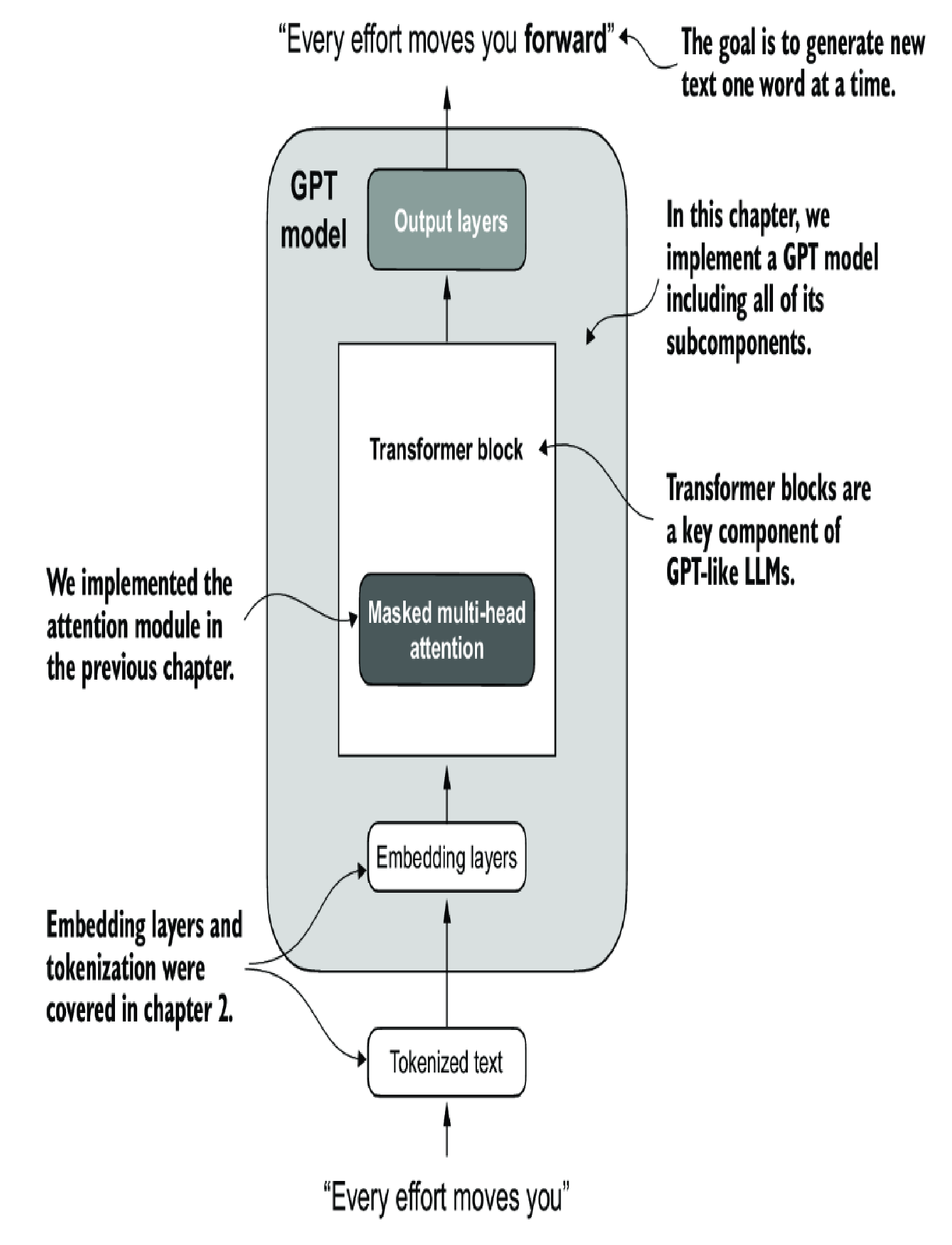
Typically, a LLM will have many blocks of Transformer (12 in above image), the output of a Transformer block will be the input of the next once in the sequence.
Layer Normalization
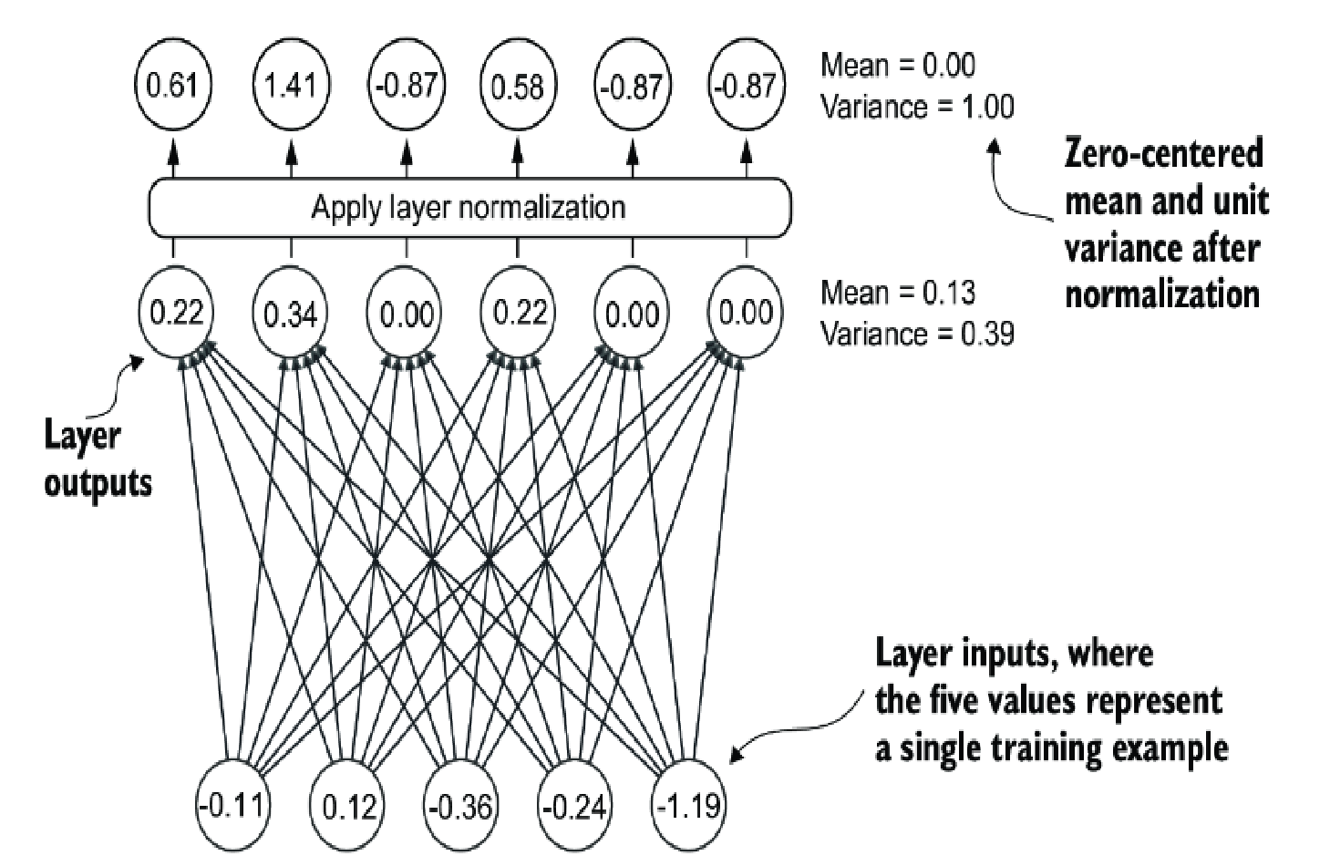
The multi-head attention is basically matrix operations to producing the context value as we discussed earlier, and those operations could produce very close to zero value or very large value after multiple layers. This is also known as vanishing gradient and exploding gradient.
This layer will make the adjustment on the parameters so that total of the value is equal to 0 (mean of 0)
\[ \mu=\frac{\sum_{i=1} ^{T}x_{i}}{T}=0 \]
and the variance of 1.
\[ \sigma ^{2} = \frac{\sum_{i=1} ^{T}(x_{i}-\mu) ^2}{T}=\frac{\sum_{i=1} ^{T}(x_{i}) ^{2}}{T}=1 \]
Vanishing gradient happens when the value is too close to zero; too many zeros after the period. The model is likely stop learning because whatever data feed in the changes is insignificant.
Exploding gradient happens when the value is too big and over the capacity of 64-bit float, it will become inf, and the next math operation on inf will become NaN and the program halts.
Runnable code
import torch
import torch.nn as nn

class LayerNorm(nn.Module):
    def __init__(self, emb_dim):
        super().__init__()
        self.eps = 1e-5
        self.scale = nn.Parameter(torch.ones(emb_dim))
        self.shift = nn.Parameter(torch.zeros(emb_dim))

    def forward(self, x):
        mean = x.mean(dim=-1, keepdim=True)
        var = x.var(dim=-1, keepdim=True, unbiased=False)
        norm_x = (x - mean) / torch.sqrt(var + self.eps)
        return self.scale * norm_x + self.shift

if __name__ == "__main__":
    # create 2 training examples with 5 dimensions (features) each
    batch_example = torch.randn(2, 5)

    ln = LayerNorm(emb_dim=5)
    out_ln = ln(batch_example)

    mean = out_ln.mean(dim=-1, keepdim=True)
    var = out_ln.var(dim=-1, unbiased=False, keepdim=True)

    print("Mean:\n", mean)
    print("Variance:\n", var)
layer_norm.py
ReLU activation
For each layer of the LLM, it will calculate the context vectors by the matrix operation, and we can think of \( y_{i+1}=W_{i+1}.y_{i} \), \( W_{i} \) is the parameter matrices we discussed earlier, and hence:
\[ y_{i+2}=W_{i+2}.y_{i+1}=W_{i+2}.(W_{i+1}.y_{i})=(W_{i+2}.W_{i+1}).y_{i}=W_{i} ^{*}.y_{i} \]
That means we can replace both \( W_{i+2} \) and \( W_{i+1} \) by a new matrix, which also means the LLM is unable to learn any new context from the data even adding as many as layers.
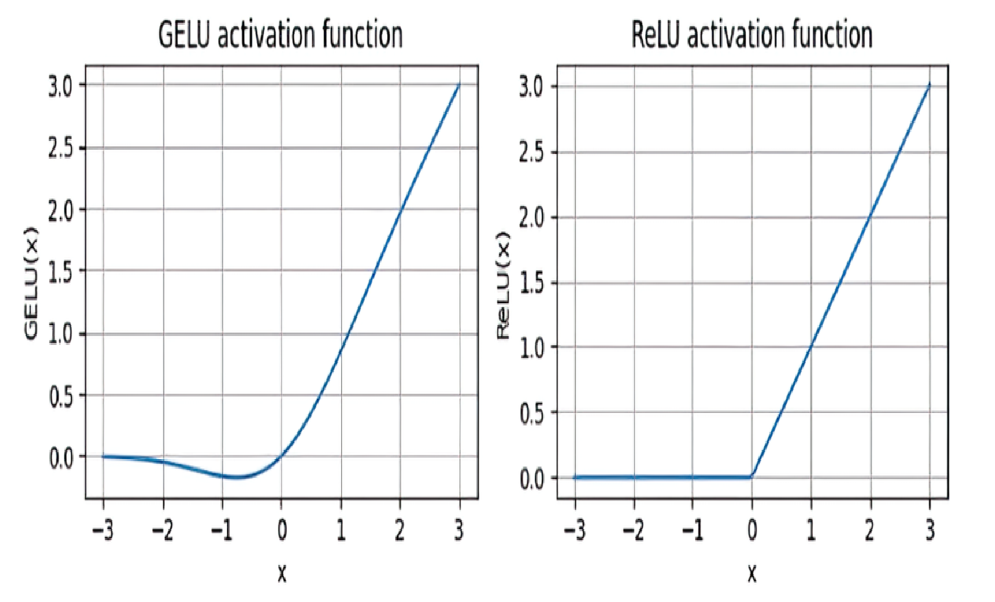
ReLU function simply turns all negative values into 0, so the chain of layers is no longer linear and creates opportunity for the LLM to learn new relationship in the input.
In reality, GELU or SwiGLU are used to have smoother activation which allows some negative inputs to contribute to learning process.
Runnable code
import torch
import torch.nn as nn

class GELU(nn.Module):
    def __init__(self):
        super().__init__()

    def forward(self, x):
        return 0.5 * x * (1 + torch.tanh(
            torch.sqrt(torch.tensor(2.0 / torch.pi)) *
            (x + 0.044715 * torch.pow(x, 3))
        ))
FeedForward module
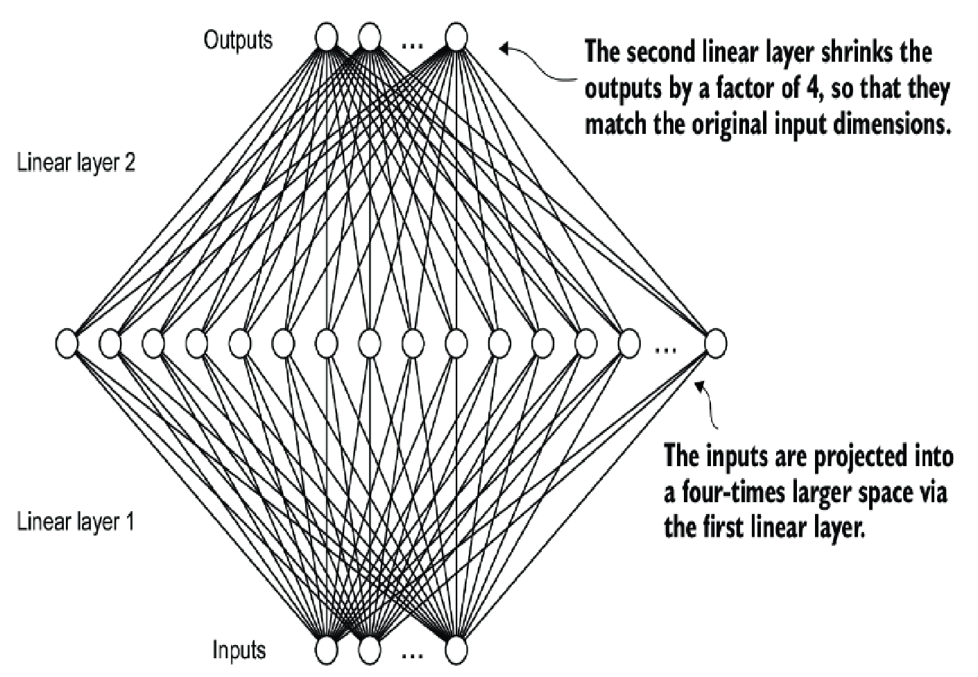
This module make an intermediate layer with significant higher number of parameters of both input and output (usually has the same size), so that the model can have ability like generalization data.
Runnable code
import torch
import torch.nn as nn
from config import GPT_CONFIG_124M
from gelu import GELU

class FeedForward(nn.Module):
    def __init__(self, cfg):
        super().__init__()
        self.layers = nn.Sequential(
            nn.Linear(cfg["emb_dim"], 4 * cfg["emb_dim"]),
            GELU(),
            nn.Linear(4 * cfg["emb_dim"], cfg["emb_dim"]),
        )

    def forward(self, x):
        return self.layers(x)

if __name__ == "__main__":
    ffn = FeedForward(GPT_CONFIG_124M)

    # input shape: [batch_size, num_token, emb_size]
    x = torch.rand(2, 3, 768)
    out = ffn(x)
    print(out.shape)
feed_forward.py
Shortcut connection
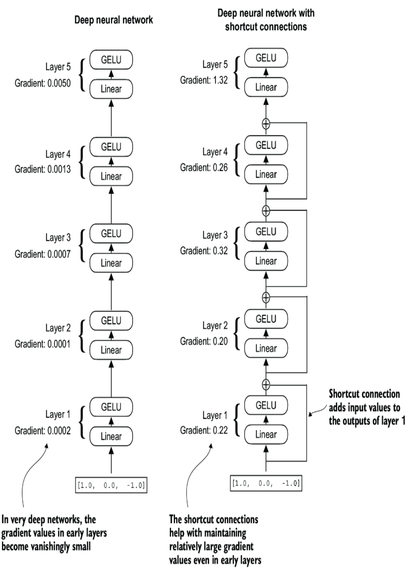
We already know the vanishing gradient and this can be happened in both ways: forward and backward propagation which means the value become too small for make signification changes. So the shortcut connection will add the input value to the output of the multi-head attention computation in order to make the output is significant again.
Don't be fooled by the the name of shortcut connection, it does not bypassing the network layer, but adding the input to the output to make more significant output values.
Transformer block
TransformerBlock class includes a multi-head attention mechanism
(MultiHeadAttention) and a feed forward network (FeedForward),
both configured based on a provided configuration dictionary
(cfg), such as GPT_CONFIG_124M. Layer normalization (LayerNorm) is applied before each of these two components, and dropout is applied after them to
regularize the model and prevent overfitting.
Runnable code
GPT_CONFIG_124M = {
    "vocab_size": 50257,    # Vocabulary size
    "context_length": 1024, # Context length
    "emb_dim": 768,         # Embedding dimension
    "n_heads": 12,          # Number of attention heads
    "n_layers": 12,         # Number of layers
    "drop_rate": 0.1,       # Dropout rate
    "qkv_bias": False       # Query-Key-Value bias
}
import torch
import torch.nn as nn
from config import GPT_CONFIG_124M
from feed_forward import FeedForward
from layer_norm import LayerNorm
from multi_head_attention import MultiHeadAttention
class TransformerBlock(nn.Module):
def __init__(self, cfg):
super().__init__()
self.att = MultiHeadAttention(
d_in=cfg["emb_dim"],
d_out=cfg["emb_dim"],
context_length=cfg["context_length"],
num_heads=cfg["n_heads"],
dropout=cfg["drop_rate"],
qkv_bias=cfg["qkv_bias"])
self.ff = FeedForward(cfg)
self.norm1 = LayerNorm(cfg["emb_dim"])
self.norm2 = LayerNorm(cfg["emb_dim"])
self.drop_shortcut = nn.Dropout(cfg["drop_rate"])
def forward(self, x):
# Shortcut connection for attention block
shortcut = x
x = self.norm1(x)
x = self.att(x) # Shape [batch_size, num_tokens, emb_size]
x = self.drop_shortcut(x)
x = x + shortcut # Add the original input back
# Shortcut connection for feed forward block
shortcut = x
x = self.norm2(x)
x = self.ff(x)
x = self.drop_shortcut(x)
x = x + shortcut # Add the original input back
return x
if __name__ == "__main__":
torch.manual_seed(123)
x = torch.rand(2, 4, 768) # Shape: [batch_size, num_tokens, emb_dim]
block = TransformerBlock(GPT_CONFIG_124M)
output = block(x)
print("Input shape:", x.shape)
print("Output shape:", output.shape)transformer.py
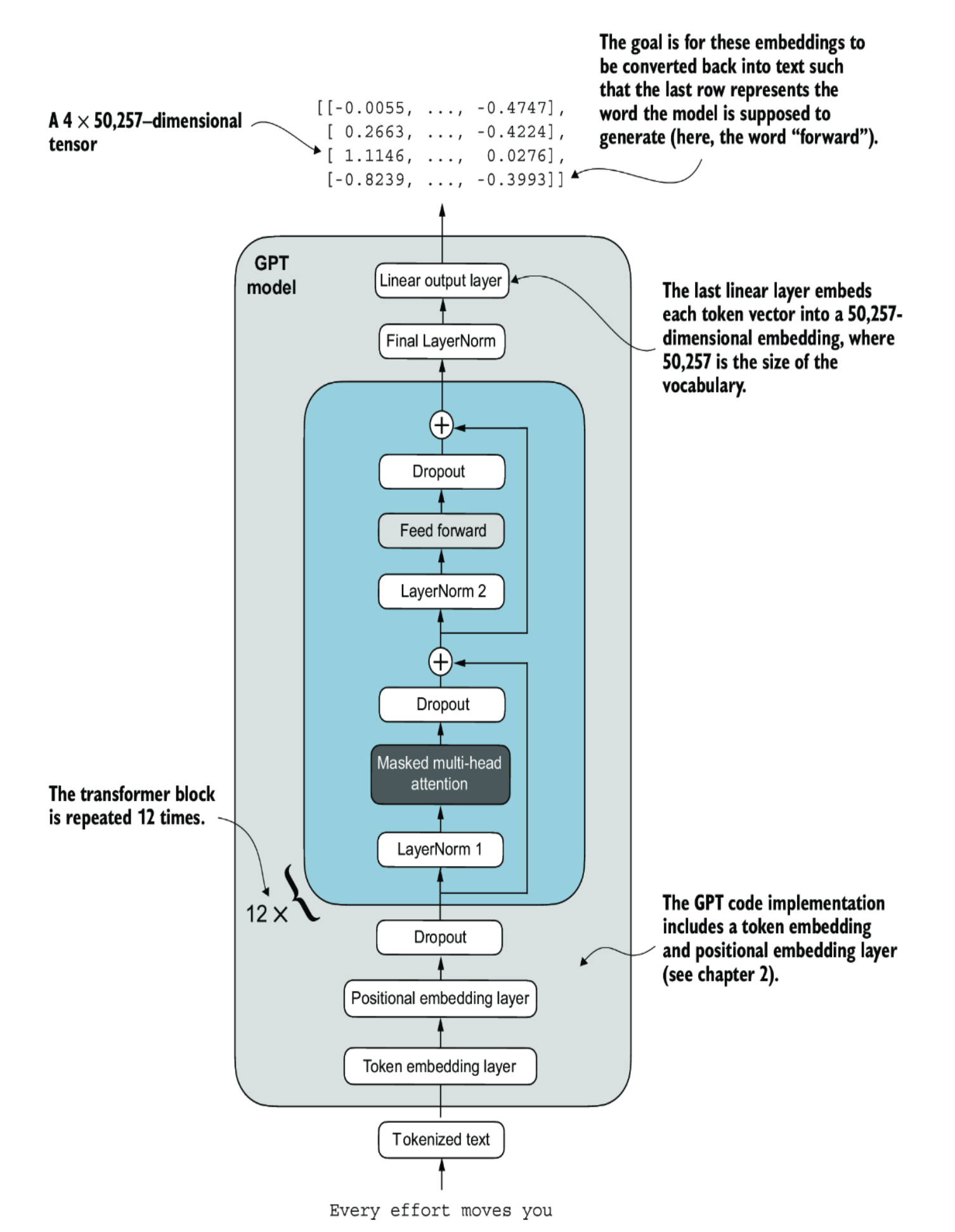
GPT code
import torch
import torch.nn as nn
import tiktoken

from config import GPT_CONFIG_124M
from layer_norm import LayerNorm
from transformer import TransformerBlock

class GPTModel(nn.Module):
    def __init__(self, cfg):
        super().__init__()
        self.tok_emb = nn.Embedding(cfg["vocab_size"], cfg["emb_dim"])
        self.pos_emb = nn.Embedding(cfg["context_length"], cfg["emb_dim"])
        self.drop_emb = nn.Dropout(cfg["drop_rate"])
        self.trf_blocks = nn.Sequential(
            *[TransformerBlock(cfg) for _ in range(cfg["n_layers"])])
        self.final_norm = LayerNorm(cfg["emb_dim"])
        self.out_head = nn.Linear(
            cfg["emb_dim"], cfg["vocab_size"], bias=False
        )

    def forward(self, in_idx):
        batch_size, seq_len = in_idx.shape
        tok_embeds = self.tok_emb(in_idx)
        #1
        pos_embeds = self.pos_emb(
            torch.arange(seq_len, device=in_idx.device)
        )
        x = tok_embeds + pos_embeds
        x = self.drop_emb(x)
        x = self.trf_blocks(x)
        x = self.final_norm(x)
        logits = self.out_head(x)
        return logits

def generate_text_simple(model, idx, #1
    max_new_tokens, context_size):
    for _ in range(max_new_tokens):
        idx_cond = idx[:, -context_size:] #2
        with torch.no_grad():
            logits = model(idx_cond)
        logits = logits[:, -1, :] #3
        probas = torch.softmax(logits, dim=-1) #4
        idx_next = torch.argmax(probas, dim=-1, keepdim=True) #5
        idx = torch.cat((idx, idx_next), dim=1) #6
    return idx

if __name__ == "__main__":

    tokenizer = tiktoken.get_encoding("gpt2")

    batch = []

    txt1 = "Every effort moves you"
    txt2 = "Every day holds a"

    batch.append(torch.tensor(tokenizer.encode(txt1)))
    batch.append(torch.tensor(tokenizer.encode(txt2)))
    batch = torch.stack(batch, dim=0)
    print(batch)

    torch.manual_seed(123)
    model = GPTModel(GPT_CONFIG_124M)

    out = model(batch)
    print("Input batch:\n", batch)
    print("\nOutput shape:", out.shape)
    print(out)

    total_params = sum(p.numel() for p in model.parameters())
    print(f"Total number of parameters: {total_params:,}")

    print("Token embedding layer shape:", model.tok_emb.weight.shape)
    print("Output layer shape:", model.out_head.weight.shape)

    total_params_gpt2 =  total_params - sum(p.numel() for p in model.out_head.parameters())
    print(f"Number of trainable parameters considering weight tying: {total_params_gpt2:,}")

    # Calculate the total size in bytes (assuming float32, 4 bytes per parameter)
    total_size_bytes = total_params * 4

    # Convert to megabytes
    total_size_mb = total_size_bytes / (1024 * 1024)

    print(f"Total size of the model: {total_size_mb:.2f} MB")

    start_context = "Hello, I am"
    encoded = tokenizer.encode(start_context)
    print("encoded:", encoded)
    encoded_tensor = torch.tensor(encoded).unsqueeze(0) #1
    print("encoded_tensor.shape:", encoded_tensor.shape)
    model.eval() #1
    out = generate_text_simple(
        model=model,
        idx=encoded_tensor,
        max_new_tokens=6,
        context_size=GPT_CONFIG_124M["context_length"]
    )
    print("Output:", out)
    print("Output length:", len(out[0]))

    decoded_text = tokenizer.decode(out.squeeze(0).tolist())
    print(decoded_text)
gpt.py


Comments ()